ML Case Study
 Photo by rawpixel on Unsplash
For data, please visit my github repo.
Case Study Overview:
Patrick, the manager of a telecommunication company wants to apply analytical techniques so that he can predict if a RF radio mast, used in mobile phone communication, is susceptible to outages due to adverse weather conditions. To this end he would like you to use appropriate algorithms and/or machine learning techniques to aid him with this task. Patrick’s company has a large nationwide network of RF radio masts and these are affected by ‘outages’ due to adverse weather conditions, mainly very heavy rain and heavy mist. Outages mean that there is no available mobile phone service. To help you Patrick has commissioned an engineer to classify 2,186 radio masts are either okay – i.e. not susceptible to adverse weather conditions and under, i.e. under engineered and so susceptible to adverse weather conditions. He has also supplied you with a scoring dataset of 936 radio masts for you to classify as whether okay or Under.
Case Study a:
Investigate the data by carrying out some Exploratory Data Analysis (EDA). Perform the necessary data cleaning/data reduction tasks.
RF Dataset
Reading the RF dataset using XLConnect package: There are two datasets i.e. Training & Scoring set. We will read both the dataset together & apply preprocessing on the combine dataset. So when we need to do prediction on scoring set, we can have prepocessed data. Training set has 2186 observation & 79 columns whereas, Scoring data set has 936 observation & 77 columns.
Exploratory Data Analysis (EDA):
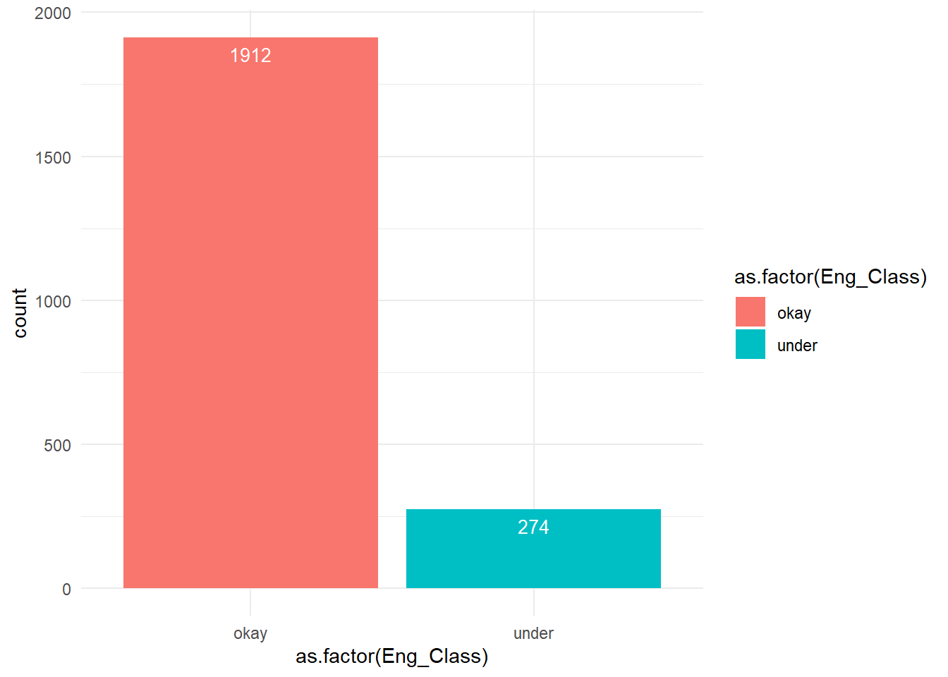
1) Response Variable Barplot: Response Variable i.e. Eng_Class has two categories i.e. okay & under. It forms an unbalanced variable distribution of 1912 into ‘okay’ & 274 into ‘under’ categories.
2) AntennagaindBi1 Variable: As can be seen from below output, there is no difference in 1st quantile & median (36.60 & 36.80). Variable is highly left skewed & there are outlier points in this variable.
##    Min. 1st Qu.  Median    Mean 3rd Qu.    Max.
##   30.90   36.60   36.80   38.05   40.10   46.70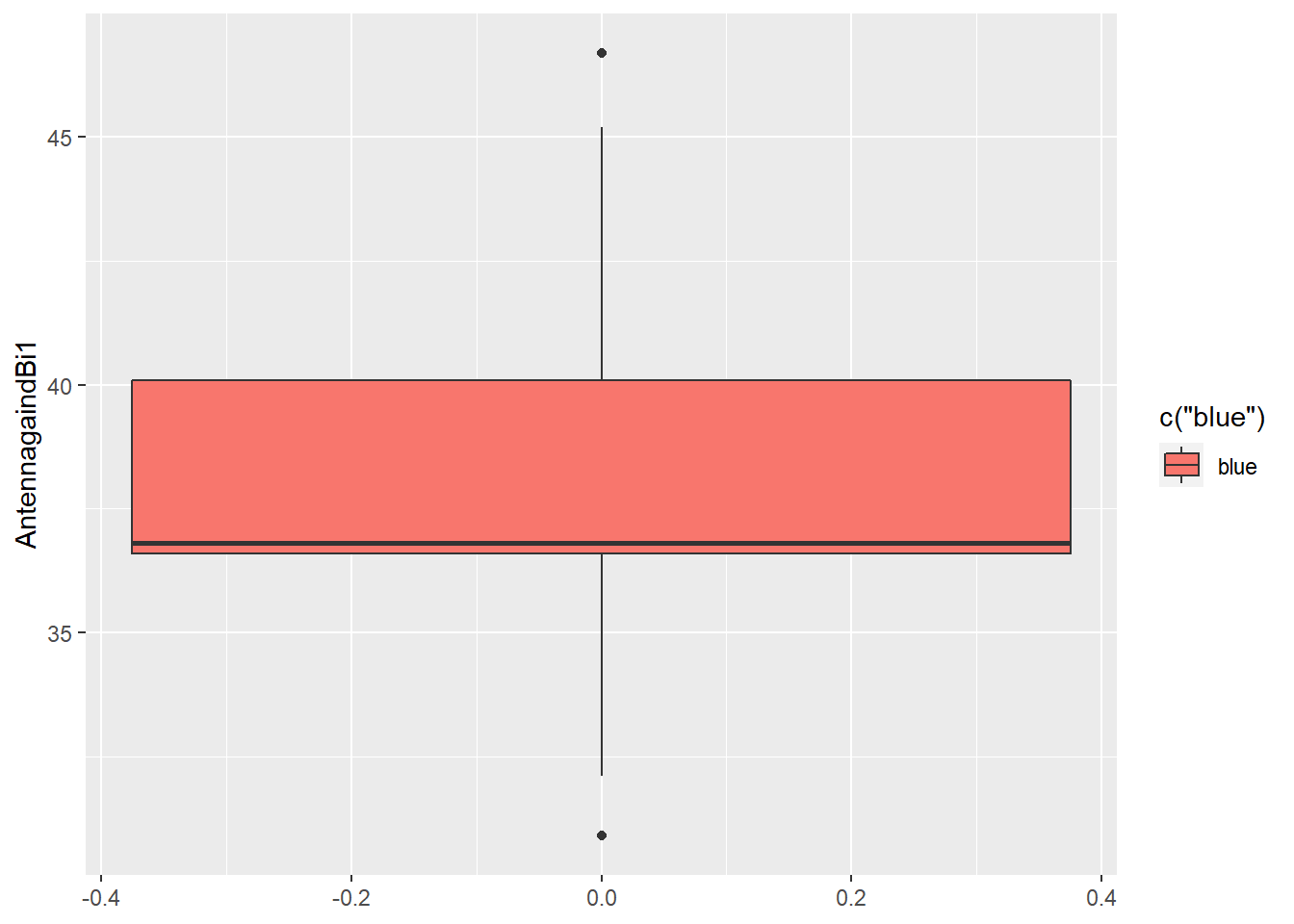
3) EIRPdBm1 Variable: These data point is left skewed. There are many lower outliers point in the variable.
##    Min. 1st Qu.  Median    Mean 3rd Qu.    Max.
##    4.10   37.10   43.80   44.56   51.80   67.20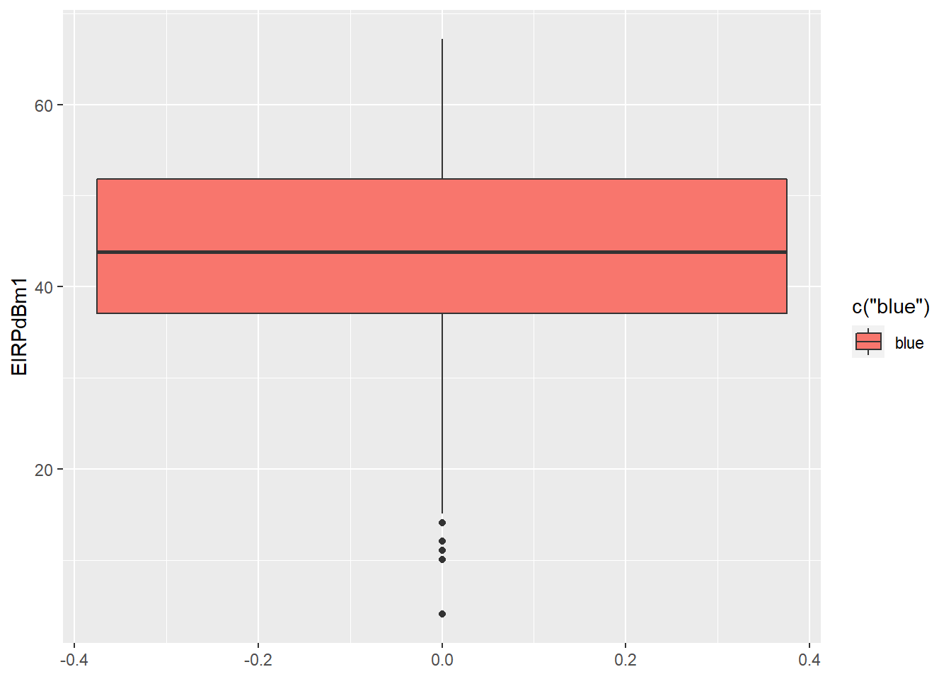
## `stat_bin()` using `bins = 30`. Pick better value with `binwidth`.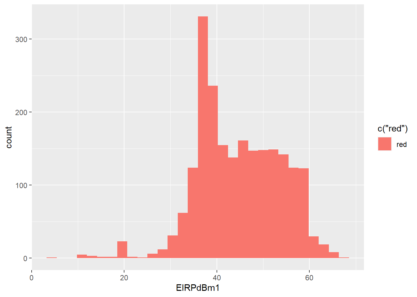
4) TXpowerdBm1 Variable: As can be seen from the below graph, these data point is left skewed. There are many lower outliers point in the variable.
##    Min. 1st Qu.  Median    Mean 3rd Qu.    Max.
##  -15.00   13.00   18.00   15.72   20.00   28.00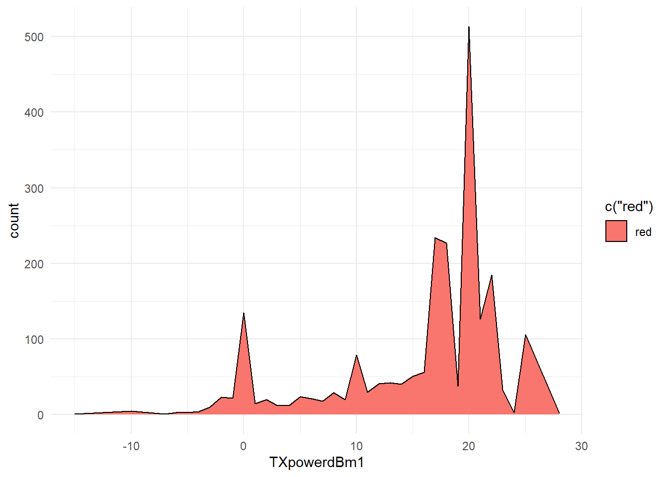
5) Polarization Variable: Variable has two categories i.e. Horizontal & Vertical. It forms an unbalanced variable distribution of 667 into ‘Horizontal’ & 1519 into ‘Vertical’ categories. Thus, attenuation factor is low as horizontal point is less.

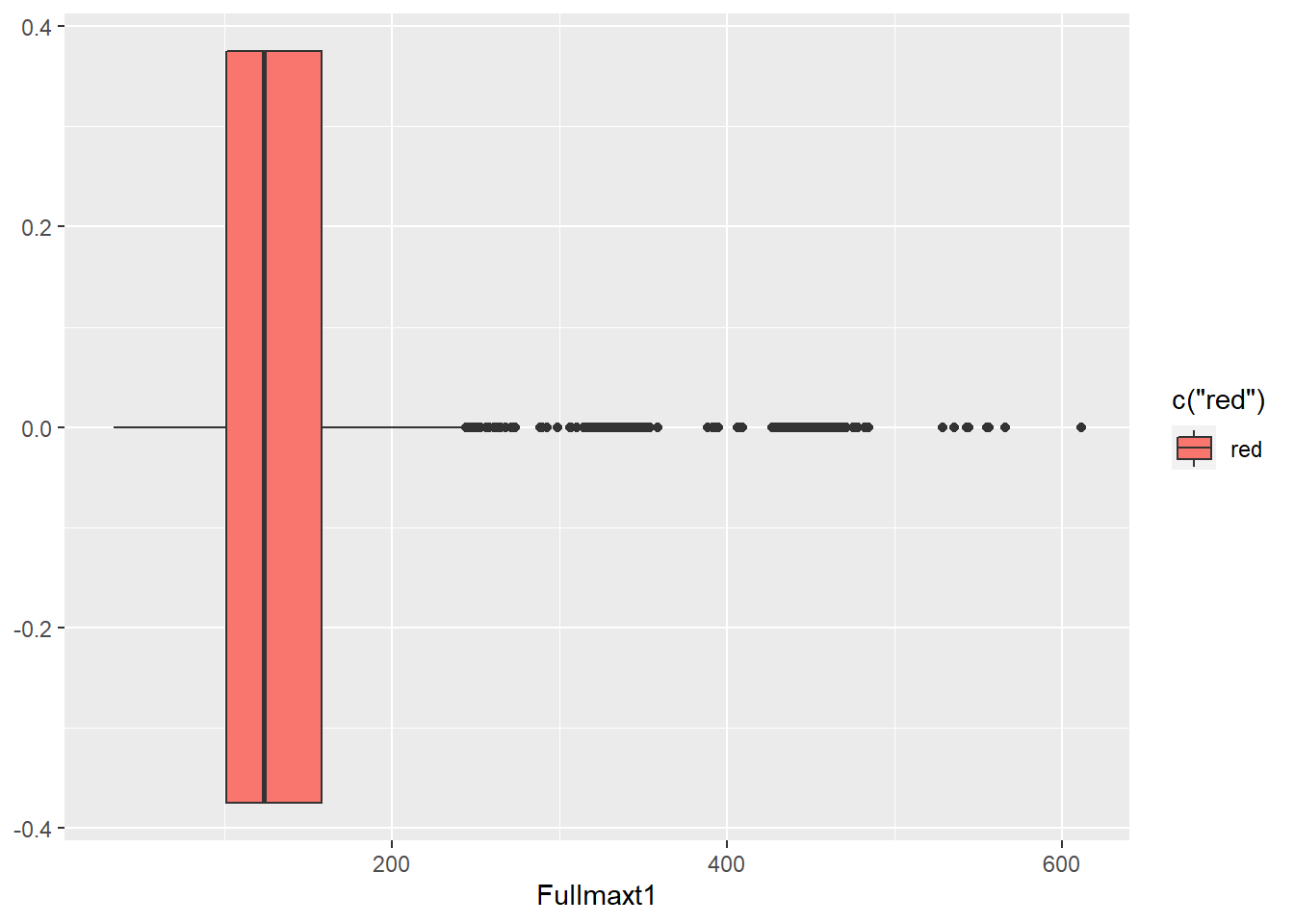
6) Fullmaxt1 Variable: These variable is right skewed. There are many upper outliers point in the variable.

## `stat_bin()` using `bins = 30`. Pick better value with `binwidth`.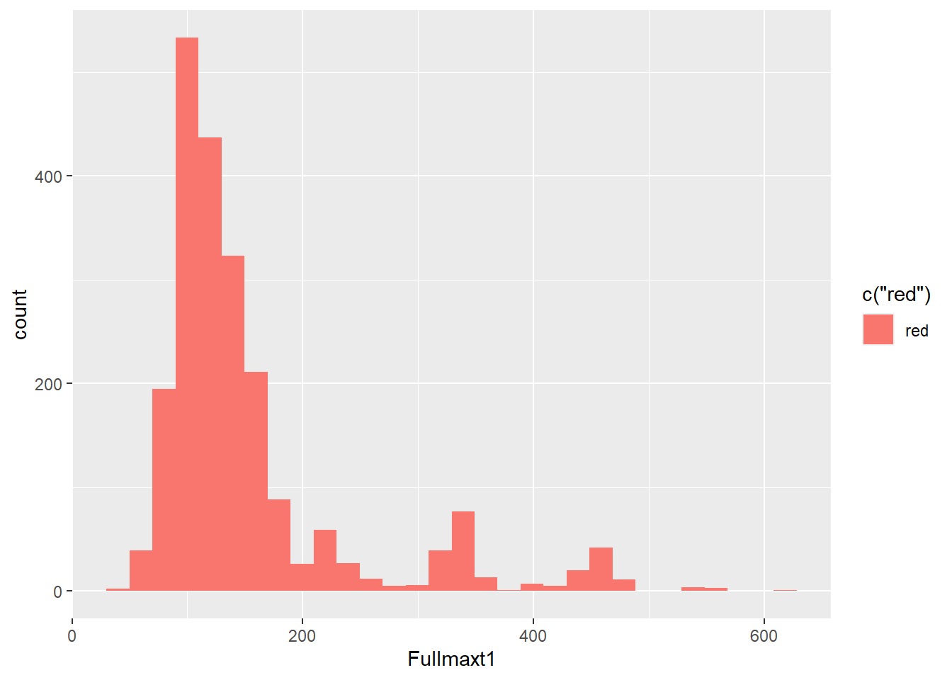
8) Summary of the dataframe: There are 21 character columns & 59 numeric columns. CirculatorbranchinglossdB1 contains all 0 value as its mean is 0. DiffractionlossdB also contains almost 0 values with a mean of 0.133 & median of 0. Only variable DpQ_R2 & Fullmint1 contains NA values._MainnetpathlossdB2_ variable is almost normally distributed. Most of the variables are skewed positively or negatively.
Glimpse of dataframe: We have quite a few variables which are character that needs to be converted to numerical. We will create dummies of such character variables & clean our data. Also, we will merge the training & Scoring dataset & preprocess them together so that we can find the prediction on scoring data without any issue.
Merging Training & Scoring set: Before merging the two dataset, we will check whether both contains the same column names or not. We can see that Scoring data set has four columns with different names (“EffectiveFadeMargindB1”,“EffectiveFadeMargindB2”,“ThermalFadeMargindB1” “ThermalFadeMargindB2”) & two columns which doesn’t exist in Scoring dataset (“Eng_Class”,“Outcome”) which is quite obvious as we need to predict Eng_Class. We will rename such columns and merge them.
Data Cleaning:
Here we will understand the dataset, remove any unwanted variables. Add more variables using dummies concept. Recreate our dataframe.
1) Removing unwanted columns: We will remove columns RFDBid, Antennafilename1, Antennafilename2 & Outcome as it will show no impact on our model.
RF_All_df1=All_RF_df %>% dplyr::select(-RFDBid,-Antennafilename1,-Antennafilename2,-Outcome)- Creating Dummies for variable Antennamodel1: As can be read in variable Antennamodel1, we have many unqiue values. If we create dummies for so many unique values of the variables, it will unnecessarily create variables which may not be impactful for our model, thus we will apply some manual analysis and accordingly create few dummies as can be read from the below line of code, we just create 4 dummies based on frequency count of character values.
test_table=sort(table(RF_All_df1$Antennamodel1),decreasing = TRUE)
RF_All_df1=RF_All_df1 %>%
  mutate(Antennamodel1_800=as.numeric(Antennamodel1 %in% names(which(test_table>800))),
         Antennamodel1_300=as.numeric(Antennamodel1 %in% names(which(test_table>300 & test_table<=800))),
         Antennamodel1_200=as.numeric(Antennamodel1 %in% names(which(test_table>200 & test_table<=300))),
         Antennamodel1_100=as.numeric(Antennamodel1 %in% names(which(test_table>100 & test_table<=200)))) %>%
dplyr::select(-Antennamodel1,-Antennamodel2)- Creating Dummies for variable Emissiondesignator1: For variable Emissiondesignator1, we will apply some manual analysis and accordingly create few dummies as can be read from the below line of code, we just create 4 dummies based on frequency count of character values. By analysis, column Emissiondesignator1 & Emissiondesignator1 contains similar records, thus we will discard one and create dummies for other.
table_emission1=sort(table(RF_All_df1$Emissiondesignator1),decreasing = TRUE)
table_emission1
##
## 28M00D7WET 56M00D7WET 7M20G7W 28M6G7W 14M2G7W 27M5D7WET 55M00D7WET
## 1535 544 397 253 112 102 99
## 3M70G7W 13M3D7W 28MG67W 56M0D7W 28M0D7W 14M0D7W
## 36 25 12 4 2 1RF_All_df1=RF_All_df1 %>%
mutate(Emissiondesignator1_1500=as.numeric(Emissiondesignator1 %in% names(which(table_emission1>1500))),
Emissiondesignator1_500=as.numeric(Emissiondesignator1 %in% names(which(table_emission1>500 & table_emission1<=1500))),
Emissiondesignator1_300=as.numeric(Emissiondesignator1 %in% names(which(table_emission1>300 & table_emission1<=500))),
Emissiondesignator1_200=as.numeric(Emissiondesignator1 %in% names(which(table_emission1>200 & table_emission1<=300)))) %>%
dplyr::select(-Emissiondesignator1,-Emissiondesignator2)- Converting Polarization categories into 1’s & 0’s: As can be read from below output, we will convert this variable into 1’s & 0’s dummy.
RF_All_df1=RF_All_df1 %>% mutate(Polarization_vertical=as.numeric(Polarization=="Vertical")) %>% dplyr::select(-Polarization)- Creating Dummies for Radiofilename1: As both column contains same value, we will remove one and we will create manual dummies for other. Here, we will create dummies based on the frequencies of the count of radiofilename.
table_radiofilename=sort(table(RF_All_df1$Radiofilename1),decreasing = TRUE)
RF_All_df1=RF_All_df1 %>%
  mutate(Radiofilename1_600=as.numeric(Radiofilename1 %in% names(which(table_radiofilename>600))),
         Radiofilename1_200=as.numeric(Radiofilename1 %in% names(which(table_radiofilename>200 & table_radiofilename<=600))),
         Radiofilename1_100=as.numeric(Radiofilename1 %in% names(which(table_radiofilename>100 & table_radiofilename<=200)))) %>%
dplyr::select(-Radiofilename1,-Radiofilename2)- Creating Dummies for Radiomodel1: As both column contains same value, we will remove one and we will create manual dummies for other based on frequency of value.
table_Radiomodel1=sort(table(RF_All_df1$Radiomodel1),decreasing = TRUE)
RF_All_df1=RF_All_df1 %>%
  mutate(Radiomodel1_300=as.numeric(Radiomodel1 %in% names(which(table_Radiomodel1>300))),
         Radiomodel1_120=as.numeric(Radiomodel1 %in% names(which(table_Radiomodel1>=120 & table_Radiomodel1<=300))),
         Radiomodel1_80=as.numeric(Radiomodel1 %in% names(which(table_Radiomodel1>=80 & table_Radiomodel1<120)))) %>%
dplyr::select(-Radiomodel1,-Radiomodel2)- Converting RXthresholdcriteria1 categories into 1’s & 0’s: As RXthresholdcriteria1 & RXthresholdcriteria1 column contains almost similar values, we will discard one and create dummy for other variables.
RF_All_df1=RF_All_df1 %>% mutate(RXthresholdcriteria_dumm1=as.numeric(RXthresholdcriteria1=="1E-6 BER")) %>%
dplyr::select(-RXthresholdcriteria1,-RXthresholdcriteria2)- Converting Character variables into numeric: As DispersivefademargindB1 variable contains numeric value in a form of characters, we will directly convert into numeric.
RF_All_df1$DispersivefademargindB1=as.numeric(RF_All_df1$DispersivefademargindB1)- Converting Character variables into numeric: As DispersivefademargindB1 variable contains numeric value in a form of characters, we will directly convert into numeric.
RF_All_df1$DispersivefademargindB1=as.numeric(RF_All_df1$DispersivefademargindB1)- Removing variables: As can be read from above output, Since the columns Passivegain2dB, MiscellaneouslossdB1, MiscellaneouslossdB2, EIRPdBm2, ERPdbm1, ERPdbm2, EffectiveFadeMargindB2, DispersivefademargindB2, MainreceivesignaldBm2, MainnetpathlossdB2, FlatfademarginmultipathdB2, OtherRXlossdB1, OtherTXlossdB2, ThermalFadeMargindB2, RXthresholdleveldBm2, RXthresholdlevelv2, TXpowerdBm2, XPDfademarginmultipathdB1 contains the same value, we will discard one and keep the other.
RF_All_df1=RF_All_df1 %>% dplyr::select(-MiscellaneouslossdB1,-MiscellaneouslossdB2,-Passivegain2dB,-EIRPdBm2,-ERPdbm1,
-ERPdbm2,-EffectiveFadeMargindB2,-DispersivefademargindB2, -MainreceivesignaldBm2,-MainnetpathlossdB2,-FlatfademarginmultipathdB2,-OtherRXlossdB1,-OtherTXlossdB2,-ThermalFadeMargindB2,-RXthresholdleveldBm2,-RXthresholdlevelv2,-TXpowerdBm2,-XPDfademarginmultipathdB1,-AntennagaindBd2)- Converting Eng_Class categories into 1’s & 0’s: Finally, converting our target variable i.e. Eng_Class into numeric.
RF_All_df1=RF_All_df1 %>% mutate(Eng_Class_new=as.numeric(Eng_Class=="okay")) %>%
dplyr::select(-Eng_Class)- Dealing with NA values: Variables Fullmint1 has 6 NA records & DpQ_R2 has 9 NA records.
##                AntennagaindBd1                AntennagaindBi1
##                              0                              0
##                AntennagaindBi2                Antennaheightm1
##                              0                              0
##                Antennaheightm2    AtmosphericabsorptionlossdB
##                              0                              0
##      AverageannualtemperatureC     CirculatorbranchinglossdB1
##                              0                              0
##     CirculatorbranchinglossdB2                   dbperKmRatio
##                              0                              0
##              DiffractionlossdB        DispersivefademargindB1
##                              0                              0
## Dispersivefadeoccurrencefactor         EffectiveFadeMargindB1
##                              0                              0
##                       EIRPdBm1                     Elevation2
##                              0                              0
##                    Elevationm1                      ERPwatts1
##                              0                              0
##                      ERPwatts2         FadeoccurrencefactorPo
##                              0                              0
##     FlatfademarginmultipathdB1                FreespacelossdB
##                              0                              0
##                   FrequencyMHz              Geoclimaticfactor
##                              0                              0
##             MainnetpathlossdB1          MainreceivesignaldBm1
##                              0                              0
##                 OtherRXlossdB2                 OtherTXlossdB1
##                              0                              0
##              Pathinclinationmr                   Pathlengthkm
##                              0                              0
##           RXthresholdleveldBm1             RXthresholdlevelv1
##                              0                              0
##           ThermalFadeMargindB1                     R_Powerfd1
##                              0                              0
##                     R_Powerfd2                   Trueazimuth1
##                              0                              0
##                   Trueazimuth2                    TXpowerdBm1
##                              0                              0
##                         DpQ_R2                 Verticalangle1
##                              9                              0
##                 Verticalangle2      XPDfademarginmultipathdB2
##                              0                              0
##                      Fullmaxt1                      Fullmint1
##                              0                              6
##                     Difference              Antennamodel1_800
##                              0                              0
##              Antennamodel1_300              Antennamodel1_200
##                              0                              0
##              Antennamodel1_100       Emissiondesignator1_1500
##                              0                              0
##        Emissiondesignator1_500        Emissiondesignator1_300
##                              0                              0
##        Emissiondesignator1_200          Polarization_vertical
##                              0                              0
##             Radiofilename1_600             Radiofilename1_200
##                              0                              0
##             Radiofilename1_100                Radiomodel1_300
##                              0                              0
##                Radiomodel1_120                 Radiomodel1_80
##                              0                              0
##      RXthresholdcriteria_dumm1                  Eng_Class_new
##                              0                            936
Thus, we will impute this variables with mean values.
RF_All_df1[which(is.na(RF_All_df1$Fullmint1)==TRUE),c('Fullmint1')]=mean(RF_All_df1$Fullmint1,na.rm = TRUE)
RF_All_df1[which(is.na(RF_All_df1$DpQ_R2)==TRUE),c('DpQ_R2')]=mean(RF_All_df1$DpQ_R2,na.rm = TRUE)
Finally, we will split our Data frame back into Training & Scoring set.
processed_training_df=RF_All_df1[which(RF_All_df1$Difference==1),!(colnames(RF_All_df1) %in% c('Difference'))]
processed_scoring_df=RF_All_df1[which(RF_All_df1$Difference==0),!(colnames(RF_All_df1) %in% c('Difference','Eng_Class_new'))]- nearZeroVar: Here, we will remove all the variables with near to zero variance. We will use function nearZeroVar() of caret.
nzv_all=nearZeroVar(processed_training_df)
nzv_train_df <- processed_training_df[,-nzv_all]
dim(nzv_train_df) #53
## [1] 2186 53- Removing highly correlated variables: In this step, we will remove all the variables with high correlation. We will use findCorrelation function and find out the variables to be removed. we have set default range to 0.75
nzv_train_Cor <- cor(nzv_train_df)
highly_CorDescr <-  findCorrelation(nzv_train_Cor, cutoff = 0.75)
cor_train_df <-  nzv_train_df[,-highly_CorDescr]
dim(cor_train_df) #39
## [1] 2186 39- Linear Dependencies: Here we will remove all the linear dependent variables. Since, we have null variables to remove i.e. we have no Linear dependencies.
LiD_train_info <-  findLinearCombos(cor_train_df)
LiD_train_info$remove
## NULLCase Study b:
Set up a training/testing methodology. Using a least 2 models, tune these models and compare your results.
Train Test Split:
Here we will split the data into training & test set.
set.seed(375)
s_1=sample(1:nrow(cor_train_df),0.7*nrow(cor_train_df))
RF_cor_train=cor_train_df[s_1,]
RF_cor_test=cor_train_df[-s_1,]
Building Model: Logistic Regression & Random Forest
Step 1) Variance Inflation Factor (VIF): Applying VIF & testing any variable above value 5. We will discard the variables with value above 5 as it can cost multicollinearity issue.
for_vif2=lm(Eng_Class_new~.,data=RF_cor_train)
RF_vars <- attributes(alias(for_vif2)$Complete)$dimnames[[1]]
RF_vars
## NULLAs can be seen from below output, variables OtherTXlossdB1, EIRPdBm1 & TXpowerdBm1 has very high VIF i.e. ranging to 1200. We will discard this variable & again check for VIF.
for_vif2=lm(Eng_Class_new~.,data=RF_cor_train)
sort(vif(for_vif2),decreasing = T)[1:3]
## OtherTXlossdB1 EIRPdBm1 TXpowerdBm1
## 1177.4690 1174.6294 773.8595As can be seen from below output, variables FrequencyMHz, FlatfademarginmultipathdB1 & Radiofilename1_600 has VIF greater than 5. Thus, we will discard this variable & again check for VIF.
for_vif2=lm(Eng_Class_new~.-OtherTXlossdB1-TXpowerdBm1-EIRPdBm1,data=RF_cor_train)
sort(vif(for_vif2),decreasing = T)[1:3]
## FrequencyMHz FlatfademarginmultipathdB1
## 8.088820 5.517495
## Radiofilename1_600
## 5.499268As can be seen from below output, we have now all VIF less than 5. Thus we will stop checking the VIF any further & proceed to build the model.
for_vif2=lm(Eng_Class_new~.-OtherTXlossdB1-TXpowerdBm1-EIRPdBm1-FrequencyMHz-FlatfademarginmultipathdB1
            -Radiofilename1_600,data=RF_cor_train)
sort(vif(for_vif2),decreasing = T)[1:3]
## Antennamodel1_800 MainnetpathlossdB1 RXthresholdcriteria_dumm1
## 3.975570 3.619529 3.263194We will remove the variables listed above & reform our data frame.
Training_model2_df=RF_cor_train %>% dplyr::select(-OtherTXlossdB1,-TXpowerdBm1,-EIRPdBm1,-FrequencyMHz,-FlatfademarginmultipathdB1,-Radiofilename1_600)
dim(Training_model2_df)
## [1] 1530 33Step 2): Building Tuned Model We will build logistic regression & random forest. Both the model been tuned parallelly as can be seen from below code. We have applied manual K-Fold logic (for loop) & during each fold, we are tunning both the model. Random forest is been tunned on mtry parameter applied on K-Fold. Logistic regression is applied to stepAIC during each fold. The best model of each Fold is predicted on test dataset & it’s metric (FScore) is calculated & thereby storing each model run data in a list.
Step 2)Best Model: The best results of each run is calculated in a list. As can be seen from below code, K-Fold tunned best model is Random forest. We will test our prediction on both the models & see the performance.
bst_index=1
final_list=list()
best_model=function(list,fscore,bst_fscore){
  for(i in 1:10){
  if(as.numeric(list[[i]][fscore])>bst_fscore){
    bst_fscore=as.numeric(list[[i]][fscore])
    bst_index=i
  }
  else{
    next
  }
  }
  final_list=list("Fscore"=bst_fscore,"Best_Index"=bst_index)
  return(final_list)
}
best_glm_model=best_model(list=glm_list,fscore="fscore_glm",bst_fscore=0)
best_rf_model=best_model(list=rf_list,fscore="fscore_rf",bst_fscore=0)

paste("Best glm score:, ",best_glm_model$Fscore)
## [1] "Best glm score:, 0.947735191637631"paste("Best glm index:, ",best_glm_model$Best_Index)## [1] "Best glm index:, 1"# paste("Cutoff:, ",glm_list[[best_glm_model$Best_Index]]['max_cutoff_glm'])
paste("rf score:, ",best_rf_model$Fscore)## [1] "rf score:, 0.955555555555556"paste("rf index:, ",best_rf_model$Best_Index)## [1] "rf index:, 7"paste("BestTune:, ",rf_list[[best_rf_model$Best_Index]]['bestTune'])## [1] "BestTune:, list(mtry = 10)"Step 4): Logistic Regression Model Performance Measurement: We will test our best Logistic Regression model on Test data. As can be seen, model is performing very good on 1’s i.e. very good precision but it is performing poorly on 0’s i.e. recall is very low.
##    0   1
## 0 58  58
## 1 22 518
## [1] "Best LR Recall: 0.5"## [1] "Best LR Precision: 0.959259259259259"Step 4): Random Forest Model Performance Measurement: We will test our best Random Forest Regression model on Test data. As can be seen, model is performing very good on 1’s i.e. very good precision & also it is performing very good on 0’s i.e. recall. This model has very high accuracy, sensitivity & a decent Kappa. Thus, after carefully building & analysing our model we will finalize our model as Random Forest.
## Confusion Matrix and Statistics
##
##           Reference
## Prediction   0   1
##          0  67   2
##          1  13 574
##
##                Accuracy : 0.9771
##                  95% CI : (0.9626, 0.9871)
##     No Information Rate : 0.878
##     P-Value [Acc > NIR] : < 2.2e-16
##
##                   Kappa : 0.8865
##
##  Mcnemar's Test P-Value : 0.009823
##
##             Sensitivity : 0.9965
##             Specificity : 0.8375
##          Pos Pred Value : 0.9779
##          Neg Pred Value : 0.9710
##              Prevalence : 0.8780
##          Detection Rate : 0.8750
##    Detection Prevalence : 0.8948
##       Balanced Accuracy : 0.9170
##
##        'Positive' Class : 1
##
## [1] "Best RF Recall: 0.971014492753623"## [1] "Best RF Precision: 0.977853492333901"## [1] "Best RF FScore: 0.823529411764706"
Question c:
Perform feature selection on your model in case study c).
Feature Selection:
Step 1): First we will do the feature selection on our best Random forest model. We will use the function important & varImpPlot of RandomForest package to understand the variable importance. As can be seen in the plot, we got MeanDecreaseGini value to decide the variable importance. We have sorted the MeanDecreaseGini column in decreasin order and accordingly rebuilding our model to find the model with minimum Out Of Bag (OOB) error.
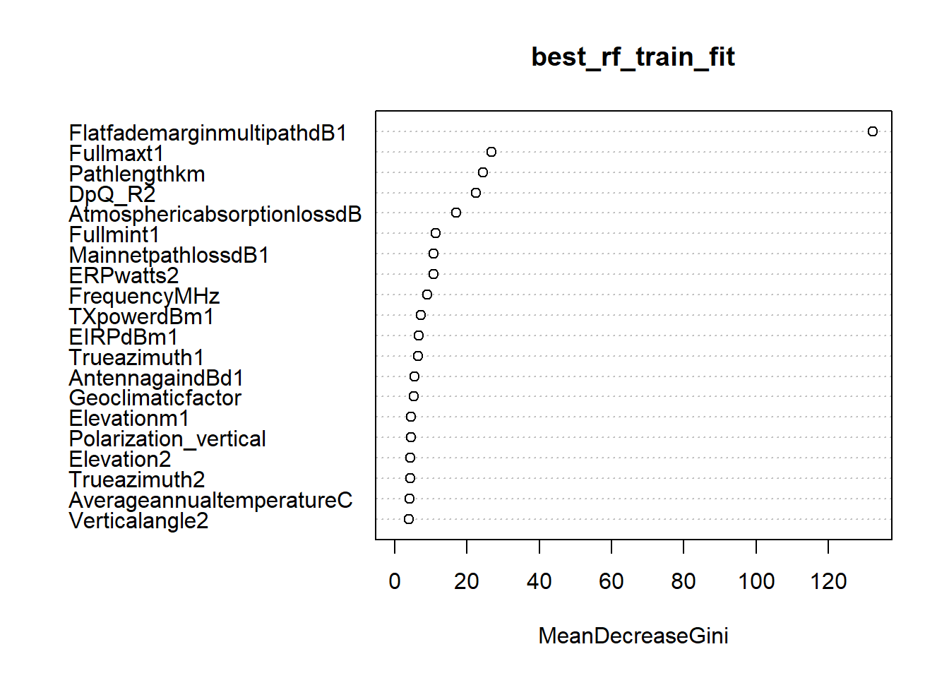
As can be learned from below output,by considering only 30 variables out of 38, we have got model OOB as 2.68% (slighyly above & below). Now, we will reduce the columns & find is there any change in OOB.
Imp_Feature_Variables=RF_Imp_df[1:20,'ColumnName']
model_formula=as.formula(paste("as.factor(Eng_Class_new)~", paste(Imp_Feature_Variables, collapse="+")))
Feature_Best_RF_Model=randomForest(model_formula,data=RF_cor_train,ntree=100,mtry=unlist(rf_list[[best_rf_model$Best_Index]]['bestTune']))
Feature_Best_RF_Model
##
## Call:
## randomForest(formula = model_formula, data = RF_cor_train, ntree = 100, mtry = unlist(rf_list[[best_rf_model$Best_Index]]["bestTune"]))
## Type of random forest: classification
## Number of trees: 100
## No. of variables tried at each split: 10
##
## OOB estimate of error rate: 3.07%
## Confusion matrix:
## 0 1 class.error
## 0 152 42 0.216494845
## 1 5 1331 0.003742515Feature_test_rf=as.numeric(as.character(unlist(predict(Feature_Best_RF_Model,newdata=RF_cor_test,type = "response"))))
Feature_ConfusionMat_rf=caret::confusionMatrix(as.factor(Feature_test_rf),as.factor(RF_cor_test$Eng_Class_new),positive="1")
best_ConfusionMat_rf## Confusion Matrix and Statistics
##
## Reference
## Prediction 0 1
## 0 67 2
## 1 13 574
##
## Accuracy : 0.9771
## 95% CI : (0.9626, 0.9871)
## No Information Rate : 0.878
## P-Value [Acc > NIR] : < 2.2e-16
##
## Kappa : 0.8865
##
## Mcnemar's Test P-Value : 0.009823
##
## Sensitivity : 0.9965
## Specificity : 0.8375
## Pos Pred Value : 0.9779
## Neg Pred Value : 0.9710
## Prevalence : 0.8780
## Detection Rate : 0.8750
## Detection Prevalence : 0.8948
## Balanced Accuracy : 0.9170
##
## 'Positive' Class : 1
## By reducing our column size to 18, we are getting least OOB i.e. 2.16% for our model. We tried many other combinations but variable with 18 gives the least OOB. Thus, we will set our feature selection to 18 columns as setted in the decreasing order based on ImpVariables.
##
## Call:
##  randomForest(formula = model_formula, data = RF_cor_train, ntree = 100,      mtry = unlist(rf_list[[best_rf_model$Best_Index]]["bestTune"]))
##                Type of random forest: classification
##                      Number of trees: 100
## No. of variables tried at each split: 10
##
##         OOB estimate of  error rate: 2.22%
## Confusion matrix:
##     0    1 class.error
## 0 164   30 0.154639175
## 1   4 1332 0.002994012
## Confusion Matrix and Statistics
##
## Reference
## Prediction 0 1
## 0 67 2
## 1 13 574
##
## Accuracy : 0.9771
## 95% CI : (0.9626, 0.9871)
## No Information Rate : 0.878
## P-Value [Acc > NIR] : < 2.2e-16
##
## Kappa : 0.8865
##
## Mcnemar's Test P-Value : 0.009823
##
## Sensitivity : 0.9965
## Specificity : 0.8375
## Pos Pred Value : 0.9779
## Neg Pred Value : 0.9710
## Prevalence : 0.8780
## Detection Rate : 0.8750
## Detection Prevalence : 0.8948
## Balanced Accuracy : 0.9170
##
## 'Positive' Class : 1
## Step 2): Second, we will apply feature selection for Logistic Regression model & see if there is any improvement in the model. We have already applied VIF (Variation Importance Factor) & stepAIC in Qb before building our model. We will see if we can go any further with StepAIC(). Here we will also apply manual feature selection based on p-value. If p-value is less than 0.05, variable is significant & it p-value is more than 0.05, variable is insignificant, we can discard such variables. If we read through the summary of the model, we can interpret that Radiomodel1_300 has the highest p-value, we will discard this column & rerun our model
##
## Call:
## glm(formula = Eng_Class_new ~ AntennagaindBd1 + AtmosphericabsorptionlossdB +
##     ERPwatts2 + MainnetpathlossdB1 + Pathlengthkm + Trueazimuth1 +
##     DpQ_R2 + Fullmaxt1 + Fullmint1 + Antennamodel1_800 + Antennamodel1_300 +
##     Antennamodel1_200 + Emissiondesignator1_500 + Emissiondesignator1_300 +
##     Emissiondesignator1_200 + Polarization_vertical + Radiomodel1_300 +
##     Radiomodel1_120, family = "binomial", data = train_data)
##
## Deviance Residuals:
##     Min       1Q   Median       3Q      Max
## -4.5982   0.0000   0.1423   0.3874   1.8176
##
## Coefficients:
##                               Estimate Std. Error z value Pr(>|z|)
## (Intercept)                 -6.042e+00  3.653e+00  -1.654 0.098109 .
## AntennagaindBd1              1.155e-01  5.527e-02   2.089 0.036679 *
## AtmosphericabsorptionlossdB -1.355e+00  2.697e-01  -5.024 5.07e-07 ***
## ERPwatts2                   -4.966e-04  3.258e-04  -1.524 0.127428
## MainnetpathlossdB1           3.085e-02  1.853e-02   1.664 0.096036 .
## Pathlengthkm                -1.034e-01  2.085e-02  -4.959 7.10e-07 ***
## Trueazimuth1                -1.480e-03  1.034e-03  -1.431 0.152366
## DpQ_R2                       1.882e-01  2.707e-02   6.955 3.53e-12 ***
## Fullmaxt1                   -1.250e-02  1.421e-03  -8.795  < 2e-16 ***
## Fullmint1                    1.829e-02  5.621e-03   3.253 0.001142 **
## Antennamodel1_800           -8.724e-01  3.772e-01  -2.312 0.020751 *
## Antennamodel1_300           -1.245e+00  6.340e-01  -1.964 0.049562 *
## Antennamodel1_200            4.651e-01  3.249e-01   1.432 0.152226
## Emissiondesignator1_500     -9.091e-01  3.248e-01  -2.799 0.005128 **
## Emissiondesignator1_300      9.758e-01  3.778e-01   2.583 0.009789 **
## Emissiondesignator1_200     -1.229e+00  3.229e-01  -3.805 0.000142 ***
## Polarization_vertical        6.571e-01  2.435e-01   2.699 0.006962 **
## Radiomodel1_300              1.580e+01  7.417e+02   0.021 0.982999
## Radiomodel1_120              1.477e+01  6.957e+02   0.021 0.983066
## ---
## Signif. codes:  0 '***' 0.001 '**' 0.01 '*' 0.05 '.' 0.1 ' ' 1
##
## (Dispersion parameter for binomial family taken to be 1)
##
##     Null deviance: 1025.40  on 1376  degrees of freedom
## Residual deviance:  598.73  on 1358  degrees of freedom
## AIC: 636.73
##
## Number of Fisher Scoring iterations: 18
## Eng_Class_new ~ AntennagaindBd1 + AtmosphericabsorptionlossdB +
## ERPwatts2 + MainnetpathlossdB1 + Pathlengthkm + Trueazimuth1 +
## DpQ_R2 + Fullmaxt1 + Fullmint1 + Antennamodel1_800 + Antennamodel1_300 +
## Antennamodel1_200 + Emissiondesignator1_500 + Emissiondesignator1_300 +
## Emissiondesignator1_200 + Polarization_vertical + Radiomodel1_300 +
## Radiomodel1_120Step 2.1): As can be seen in the output summary, Radiomodel1_120 has the highest p-value of 0.982268. we will discard this variable & rerun our model.
##
## Call:
## glm(formula = as.factor(Eng_Class_new) ~ AntennagaindBd1 + AtmosphericabsorptionlossdB +
##     ERPwatts2 + MainnetpathlossdB1 + Pathlengthkm + Trueazimuth1 +
##     DpQ_R2 + Fullmaxt1 + Fullmint1 + Antennamodel1_800 + Antennamodel1_300 +
##     Antennamodel1_200 + Emissiondesignator1_500 + Emissiondesignator1_300 +
##     Emissiondesignator1_200 + Polarization_vertical + Radiomodel1_120,
##     family = "binomial", data = RF_cor_train)
##
## Deviance Residuals:
##     Min       1Q   Median       3Q      Max
## -4.5676   0.0004   0.1876   0.4091   2.2938
##
## Coefficients:
##                               Estimate Std. Error z value Pr(>|z|)
## (Intercept)                 -8.634e+00  3.270e+00  -2.641 0.008275 **
## AntennagaindBd1              1.392e-01  5.077e-02   2.743 0.006093 **
## AtmosphericabsorptionlossdB -1.351e+00  2.370e-01  -5.700 1.20e-08 ***
## ERPwatts2                   -4.556e-04  2.833e-04  -1.608 0.107865
## MainnetpathlossdB1           5.328e-02  1.658e-02   3.214 0.001308 **
## Pathlengthkm                -1.071e-01  1.921e-02  -5.578 2.43e-08 ***
## Trueazimuth1                -7.673e-04  9.541e-04  -0.804 0.421240
## DpQ_R2                       1.900e-01  2.438e-02   7.793 6.52e-15 ***
## Fullmaxt1                   -1.192e-02  1.296e-03  -9.193  < 2e-16 ***
## Fullmint1                    1.843e-02  5.180e-03   3.559 0.000373 ***
## Antennamodel1_800           -6.200e-01  3.352e-01  -1.850 0.064328 .
## Antennamodel1_300           -1.830e+00  5.399e-01  -3.390 0.000700 ***
## Antennamodel1_200            5.082e-01  2.999e-01   1.695 0.090144 .
## Emissiondesignator1_500     -8.165e-01  2.988e-01  -2.733 0.006278 **
## Emissiondesignator1_300      7.147e-01  3.414e-01   2.093 0.036312 *
## Emissiondesignator1_200     -1.255e+00  3.002e-01  -4.181 2.90e-05 ***
## Polarization_vertical        5.474e-01  2.245e-01   2.438 0.014766 *
## Radiomodel1_120              1.480e+01  6.657e+02   0.022 0.982268
## ---
## Signif. codes:  0 '***' 0.001 '**' 0.01 '*' 0.05 '.' 0.1 ' ' 1
##
## (Dispersion parameter for binomial family taken to be 1)
##
##     Null deviance: 1163.57  on 1529  degrees of freedom
## Residual deviance:  718.88  on 1512  degrees of freedom
## AIC: 754.88
##
## Number of Fisher Scoring iterations: 18
Step 2.2): As can be seen in the output summary, ERPwatts2 has the highest p-value of 0.109130. We will discard this variable & rerun our model.
##
## Call:
## glm(formula = as.factor(Eng_Class_new) ~ AntennagaindBd1 + AtmosphericabsorptionlossdB +
##     ERPwatts2 + MainnetpathlossdB1 + Pathlengthkm + Trueazimuth1 +
##     DpQ_R2 + Fullmaxt1 + Fullmint1 + Antennamodel1_800 + Antennamodel1_300 +
##     Antennamodel1_200 + Emissiondesignator1_500 + Emissiondesignator1_300 +
##     Emissiondesignator1_200 + Polarization_vertical, family = "binomial",
##     data = RF_cor_train)
##
## Deviance Residuals:
##     Min       1Q   Median       3Q      Max
## -4.6191   0.0274   0.1959   0.4068   2.3107
##
## Coefficients:
##                               Estimate Std. Error z value Pr(>|z|)
## (Intercept)                 -8.5003691  3.2678535  -2.601 0.009290 **
## AntennagaindBd1              0.1377780  0.0508584   2.709 0.006748 **
## AtmosphericabsorptionlossdB -1.3727265  0.2374566  -5.781 7.43e-09 ***
## ERPwatts2                   -0.0004563  0.0002848  -1.602 0.109130
## MainnetpathlossdB1           0.0512612  0.0164231   3.121 0.001801 **
## Pathlengthkm                -0.1082648  0.0192016  -5.638 1.72e-08 ***
## Trueazimuth1                -0.0007746  0.0009541  -0.812 0.416864
## DpQ_R2                       0.1924879  0.0243624   7.901 2.77e-15 ***
## Fullmaxt1                   -0.0121036  0.0012963  -9.337  < 2e-16 ***
## Fullmint1                    0.0182351  0.0051793   3.521 0.000430 ***
## Antennamodel1_800           -0.5554381  0.3326402  -1.670 0.094962 .
## Antennamodel1_300           -1.8677954  0.5412254  -3.451 0.000558 ***
## Antennamodel1_200            0.5003826  0.3008147   1.663 0.096227 .
## Emissiondesignator1_500     -0.8798218  0.2976097  -2.956 0.003114 **
## Emissiondesignator1_300      0.6943934  0.3420796   2.030 0.042365 *
## Emissiondesignator1_200     -1.3031044  0.3001923  -4.341 1.42e-05 ***
## Polarization_vertical        0.5539652  0.2242011   2.471 0.013480 *
## ---
## Signif. codes:  0 '***' 0.001 '**' 0.01 '*' 0.05 '.' 0.1 ' ' 1
##
## (Dispersion parameter for binomial family taken to be 1)
##
##     Null deviance: 1163.57  on 1529  degrees of freedom
## Residual deviance:  722.76  on 1513  degrees of freedom
## AIC: 756.76
##
## Number of Fisher Scoring iterations: 8
Step 2.3): As can be seen in the output summary, Trueazimuth1 has the highest p-value of 0.416864. We will discard this variable & rerun our model.
##
## Call:
## glm(formula = as.factor(Eng_Class_new) ~ AntennagaindBd1 + AtmosphericabsorptionlossdB +
##     MainnetpathlossdB1 + Pathlengthkm + ERPwatts2 + DpQ_R2 +
##     Fullmaxt1 + Fullmint1 + Antennamodel1_800 + Antennamodel1_300 +
##     Antennamodel1_200 + Emissiondesignator1_500 + Emissiondesignator1_300 +
##     Emissiondesignator1_200 + Polarization_vertical, family = "binomial",
##     data = RF_cor_train)
##
## Deviance Residuals:
##     Min       1Q   Median       3Q      Max
## -4.6114   0.0275   0.1973   0.4016   2.2565
##
## Coefficients:
##                               Estimate Std. Error z value Pr(>|z|)
## (Intercept)                 -8.6760832  3.2594708  -2.662 0.007772 **
## AntennagaindBd1              0.1378977  0.0508576   2.711 0.006699 **
## AtmosphericabsorptionlossdB -1.3877626  0.2368105  -5.860 4.62e-09 ***
## MainnetpathlossdB1           0.0507829  0.0164219   3.092 0.001986 **
## Pathlengthkm                -0.1086071  0.0191887  -5.660 1.51e-08 ***
## ERPwatts2                   -0.0004520  0.0002845  -1.589 0.112094
## DpQ_R2                       0.1931172  0.0243136   7.943 1.98e-15 ***
## Fullmaxt1                   -0.0120321  0.0012902  -9.326  < 2e-16 ***
## Fullmint1                    0.0179437  0.0051531   3.482 0.000497 ***
## Antennamodel1_800           -0.5791253  0.3308041  -1.751 0.080005 .
## Antennamodel1_300           -1.8906320  0.5397870  -3.503 0.000461 ***
## Antennamodel1_200            0.4839706  0.2999338   1.614 0.106616
## Emissiondesignator1_500     -0.9036797  0.2965588  -3.047 0.002310 **
## Emissiondesignator1_300      0.6948596  0.3420784   2.031 0.042226 *
## Emissiondesignator1_200     -1.3177505  0.2989810  -4.407 1.05e-05 ***
## Polarization_vertical        0.5521965  0.2241849   2.463 0.013773 *
## ---
## Signif. codes:  0 '***' 0.001 '**' 0.01 '*' 0.05 '.' 0.1 ' ' 1
##
## (Dispersion parameter for binomial family taken to be 1)
##
##     Null deviance: 1163.57  on 1529  degrees of freedom
## Residual deviance:  723.42  on 1514  degrees of freedom
## AIC: 755.42
##
## Number of Fisher Scoring iterations: 8
Step 2.4): As can be seen in the output summary, ERPwatts2 has the highest p-value of 0.112094. We will discard this variable & rerun our model.
##
## Call:
## glm(formula = as.factor(Eng_Class_new) ~ AntennagaindBd1 + AtmosphericabsorptionlossdB +
##     MainnetpathlossdB1 + Pathlengthkm + DpQ_R2 + Fullmaxt1 +
##     Fullmint1 + Antennamodel1_800 + Antennamodel1_300 + Antennamodel1_200 +
##     Emissiondesignator1_500 + Emissiondesignator1_300 + Emissiondesignator1_200 +
##     Polarization_vertical, family = "binomial", data = RF_cor_train)
##
## Deviance Residuals:
##     Min       1Q   Median       3Q      Max
## -4.5202   0.0296   0.2019   0.4043   2.2619
##
## Coefficients:
##                              Estimate Std. Error z value Pr(>|z|)
## (Intercept)                 -8.214678   3.250452  -2.527 0.011496 *
## AntennagaindBd1              0.134809   0.050968   2.645 0.008170 **
## AtmosphericabsorptionlossdB -1.408581   0.237028  -5.943 2.80e-09 ***
## MainnetpathlossdB1           0.048836   0.016368   2.984 0.002848 **
## Pathlengthkm                -0.117455   0.018282  -6.425 1.32e-10 ***
## DpQ_R2                       0.185787   0.023624   7.864 3.71e-15 ***
## Fullmaxt1                   -0.012021   0.001289  -9.326  < 2e-16 ***
## Fullmint1                    0.017039   0.005100   3.341 0.000835 ***
## Antennamodel1_800           -0.620361   0.329125  -1.885 0.059446 .
## Antennamodel1_300           -1.926204   0.539441  -3.571 0.000356 ***
## Antennamodel1_200            0.482937   0.299452   1.613 0.106801
## Emissiondesignator1_500     -0.964910   0.295167  -3.269 0.001079 **
## Emissiondesignator1_300      0.706511   0.341326   2.070 0.038461 *
## Emissiondesignator1_200     -1.301462   0.296999  -4.382 1.18e-05 ***
## Polarization_vertical        0.586247   0.222917   2.630 0.008541 **
## ---
## Signif. codes:  0 '***' 0.001 '**' 0.01 '*' 0.05 '.' 0.1 ' ' 1
##
## (Dispersion parameter for binomial family taken to be 1)
##
##     Null deviance: 1163.57  on 1529  degrees of freedom
## Residual deviance:  725.83  on 1515  degrees of freedom
## AIC: 755.83
##
## Number of Fisher Scoring iterations: 8
Step 2.5): As can be seen from below output summary, all the variables are now significant. Thus, we will stop removing any further features & build our model on this features. We will check the model performance on this many features.
##
## Call:
## glm(formula = as.factor(Eng_Class_new) ~ AntennagaindBd1 + AtmosphericabsorptionlossdB +
##     MainnetpathlossdB1 + Pathlengthkm + DpQ_R2 + Fullmaxt1 +
##     Fullmint1 + Antennamodel1_800 + Antennamodel1_300 + Emissiondesignator1_500 +
##     Emissiondesignator1_300 + Emissiondesignator1_200 + Polarization_vertical,
##     family = "binomial", data = RF_cor_train)
##
## Deviance Residuals:
##     Min       1Q   Median       3Q      Max
## -4.5070   0.0294   0.2028   0.4041   2.2520
##
## Coefficients:
##                              Estimate Std. Error z value Pr(>|z|)
## (Intercept)                 -8.001393   3.256954  -2.457 0.014022 *
## AntennagaindBd1              0.122011   0.050339   2.424 0.015359 *
## AtmosphericabsorptionlossdB -1.403087   0.236422  -5.935 2.94e-09 ***
## MainnetpathlossdB1           0.052142   0.016286   3.202 0.001367 **
## Pathlengthkm                -0.121511   0.018116  -6.707 1.98e-11 ***
## DpQ_R2                       0.187723   0.023653   7.936 2.08e-15 ***
## Fullmaxt1                   -0.012195   0.001288  -9.466  < 2e-16 ***
## Fullmint1                    0.016311   0.005057   3.225 0.001258 **
## Antennamodel1_800           -0.799058   0.313236  -2.551 0.010742 *
## Antennamodel1_300           -2.097290   0.533630  -3.930 8.49e-05 ***
## Emissiondesignator1_500     -1.024058   0.294861  -3.473 0.000515 ***
## Emissiondesignator1_300      0.804835   0.333038   2.417 0.015664 *
## Emissiondesignator1_200     -1.325079   0.295964  -4.477 7.56e-06 ***
## Polarization_vertical        0.593235   0.222522   2.666 0.007677 **
## ---
## Signif. codes:  0 '***' 0.001 '**' 0.01 '*' 0.05 '.' 0.1 ' ' 1
##
## (Dispersion parameter for binomial family taken to be 1)
##
##     Null deviance: 1163.57  on 1529  degrees of freedom
## Residual deviance:  728.48  on 1516  degrees of freedom
## AIC: 756.48
##
## Number of Fisher Scoring iterations: 8
Rebuilding our Logistic regression model based on feature selection has brought a slight improvement in the model performance. We can see that 0’s ratio has improved a bit. But overall, still Random forest performs better.
##    0   1
## 0 60  59
## 1 20 517
## [1] "Best LR Recall: 0.513513513513513"## [1] "Best LR Precision: 0.957798165137615"Case Study d:
For your best model explain to Patrick how this model works. Give and explain the cost/loss function used in your modelling.
Model Explanation & Cost/Loss Function:
As we can see that, our best model is Random Forest after finely tuning & running over K-Fold validation. We also verified the best model on feature selection using variance importance technique. We got OOB for our model near to 2%. We analyzed our best model based on F1Score metric which is a trade off between recall & precision.
Basically, Random forest uses multiple decision tree in background to fit the best model. Decision tree has three nodes namely parent node, root node & terminal node. Decision tree uses any one of three metrics i.e. Gini index, Entropy, Information gain to split the data. We will consider the metric Entropy to decide the splitting of the data. In Random forest, the number of variables required for a single tree is decided using the formula √P where P is the number of variables that complete dataset has. Once the variable count is known for a single tree, Random forest will randomly choose that many variables from the whole column list & it will randomly split the data into train & test observations required in a single decision tree. We give training dataset to random forest, random forest itself further splits this data into train & test randomly for each decision tree. It builds the tree on train set & test its result on test set. Thus, random in random forest is the random variables & random train test split required to process a single tree. For e.g. if we have 9 columns & 100 observations, it will choose √9=3 variables & split 100 observation into 70% train set & 30% test set for a tree randomly. In decision tree, the first node column is chosen based on Entropy. Column with a lower entropy is chosen & splits the data into either True or False sub node also called as root node. Further splitting of the data is done with respect to column with a lowest entropy. This splitting repeat based on the size of the tree decided during parameter of Random forest.
Considering all the decision tree is formed based on the parameter ntree i.e. number of trees our random forest generates, now the random forest takes the final decision of classification based on highest category voting. For instance, if we have ntree as 500 & assuming 290 tree gives result as ‘okay’ & 210 tree gives result as ‘under’, the category with highest count is chosen i.e. okay. The process of voting repeats for all the data points. Each tree generates the error known as Out Of Bag error (OOB). This error reduces with each tree. Random forest finally generates the confusion matrix on the complete training set. Cost or Loss function is the misclassification error term. Machine learning algorithms are trained to minimize the cost function. The difference in cost & loss function is that cost function is for whole observation whereas loss is considered for one particular observation. Cost function used in classification is different than used in regression. In regression, the main idea of Cost function (MSE) is to reduce the error term by optimizing the value of weight (beta). We consider the algorithm Gradient descent to reduce the error by optimizing the value of beta. During each descent, we multiply previous slope value with the learning rate.
In classification, cross entropy cost function is used to measure the distance between two probability distributions [1]. As we know that in classification problem, we get probability value & the class with highest probability is selected as the winning prediction. The model adjusts its weight when the predicted probability is far from the actual one. Cross entropy is used to calculate the measure of predicted probability from actual one. Considering the probability distribution for two classes i.e. okay & under [1].
P(D) = [y(okay’), y(under’)]
A(D) = [y(okay), y(under)]
Cross entropy is calculated as [1]
CrossEntropy=-(okay * log(okay’) + under * log(under’))
If we consider the below predicted & actual outcome,
p(okay) = [0.8,0.2]
A(okay) = [1,0]
Our cross entropy will be,
Cross_Entropy = - (1 * log (0.8) + 0 * log (0.2)) = 0.2231436
Our model has only two classes namely okay & under. we will use Binary cross entropy cost function.
When the category is 1 i.e. okay [1],
cross_entropy=-y*log(y’)
& when the category is 0 i.e. under [1],
cross_entropy=-(1-y) * log (1-y’)
The error in binary classification is given by below formula [1]
Binary cross entropy= (sum of cross entropy for N observation)/N
Binary cross entropy penalizes if the prediction is wrongly measured [1]. For both the categories i.e. y=1 (okay) & y=1 (under), cost function reaches infinity when predicted probability is wrongly interpreted. Therefore, cross entropy is considered as the good metric for classification problem as it penalizes the wrong prediction [1].
Case Study e:
Patrick is primarily concerned with finding the under engineered masts as these are the ones that cause outages, so incorrectly ‘scoring’ a mast as under when is it okay is not as bad as incorrectly ‘scoring’ a mast as okay when it is under; you can take the ratio here of misclassification ‘costs’ as 1:h, where h = {8, 16, 24}, i.e. h can take a value of 8, 16 or 24. Redo your modelling using your best model above.
Misclassification ratio 1:h where h={8,16,24}:
Cost ratio is a ratio of False Positive (FP) cost to the False Negative (FN) cost [2]. A cost ratio of 1:8 means that cost of a False Negative (expected ‘okay’ predicted ‘under’) is eigt times that of a false positive (expected ‘under’ predicted ‘okay’). As per the business requirements, we want incorrect scoring of okay when it is under should be less. Thus, we will assign more weight to it so as to reduce the error of False Positive. We judge the classifier on total cost calculated as __Total_cost = FP* FP(cost) + FN*FN(cost)__[2].
Model with cost ratio 1:8:
Here, we will apply the cost matrix and past as a parameter to our best Random Forest model. We will keep the cost ratio as 1:8 & pass to a small simulation function which gives the best ratio of FP/FN for our cost matrix. As can be seen from the rest, we have got the ratio as 5/40 which is exacly as 1/8.
cost_ratio(h=8)##
## Call:
## randomForest(formula = model_formula, data = RF_cor_train, ntree = 100, mtry = unlist(rf_list[[best_rf_model$Best_Index]]["bestTune"]), parms = list(loss = costMatrix))
## Type of random forest: classification
## Number of trees: 100
## No. of variables tried at each split: 10
##
## OOB estimate of error rate: 2.35%
## Confusion matrix:
## 0 1 class.error
## 0 162 32 0.164948454
## 1 4 1332 0.002994012Model with cost ratio 1:16:
Here, We will keep the cost ratio as 1:16 & pass to a small simulation function which gives the best ratio of FP/FN for our cost matrix. As can be seen from the rest, we have got the ratio as 2/34 which is approximately equal to 1/16.
cost_ratio(h=16)##
## Call:
## randomForest(formula = model_formula, data = RF_cor_train, ntree = 100, mtry = unlist(rf_list[[best_rf_model$Best_Index]]["bestTune"]), parms = list(loss = costMatrix))
## Type of random forest: classification
## Number of trees: 100
## No. of variables tried at each split: 10
##
## OOB estimate of error rate: 2.42%
## Confusion matrix:
## 0 1 class.error
## 0 161 33 0.170103093
## 1 4 1332 0.002994012Model with cost ratio 1:24:
Here, We will keep the cost ratio as 1:24. Model result for this ratio is not that accurate compare to previous 2 results for h={8,16}.
costMatrix <- matrix(c(0,1,24,0), nrow=2)
    best_24_model=randomForest(model_formula, data = RF_cor_train, ntree = 100,mtry= unlist(rf_list[[best_rf_model$Best_Index]]['bestTune']),parms = list(loss=costMatrix))
    best_24_model
##
## Call:
## randomForest(formula = model_formula, data = RF_cor_train, ntree = 100, mtry = unlist(rf_list[[best_rf_model$Best_Index]]["bestTune"]), parms = list(loss = costMatrix))
## Type of random forest: classification
## Number of trees: 100
## No. of variables tried at each split: 10
##
## OOB estimate of error rate: 2.61%
## Confusion matrix:
## 0 1 class.error
## 0 158 36 0.185567010
## 1 4 1332 0.002994012Case Study f:
Using the scoring data set provided predict whether these radio masts will be okay or under engineered using your best model to part d) and comment.
Prediction on Scoring data:
As we have already preprocessed our Scoring dataframe parallely with our Training dataset. Here, we need to use our best model & predict the outcome. Our best model was Random forest applied on feature selection. We cannot estimate any model metric as we don’t have any actual y i.e. Eng_Class variable. We can read from below distribution of 1’s & 0’s from below output.
Scoring_Prediction=as.numeric(as.character(unlist(predict(Feature_Best_RF_Model,newdata=processed_scoring_df,type = "response"))))
table(Scoring_Prediction)
## Scoring_Prediction
## 0 1
## 104 832Case Study g (i):
Convolutional Neural Network Overview:
Convolutional Neural Network made up of neurons with weights & biases as learnable parameter [3]. It’s base architecture follows basic neural network. The added advantage of using CNN over basic Neural Network is considering the fact of neurons size. Suppose for an image data, we have 26 * 26 size i.e. 676 size, such size of neurons are adaptable to basic neural network system but what if we have a neural network of size 800*800. For such size, its operation processing would be very high [3]. Thus, CNN is used in such cases where it does feature extraction and convert into lower dimension without lossing its important characteristics.
Image data constitute of 3 dimensional data points i.e. height, length & the color. CNN has hidden layer as convolution layer which is used to detect patterns in the images & it is the feature extracting layer [3]. For each convolution layer, it is important to define the number of filters that the layer should contain. It is the filter that detects the sophisticated patterns in the image. Filter consist of a small matrix whose values are initialize by random numbers. If we set filter size as 3 * 3, it will stride over 3 * 3 size image & apply dot product & store its value in a single size data point. It extracts the image features part by part by calculating dot product between receptive field & the filter [4]. It repeats the process untill all the field is completed. The receptive field is decided based on the field size matrix, it stride & repeat the operation.
Convolution layer output is passed to the input of Pooling layer. Max pooling reduces the dimensionality of the images by reducing the number of pixels. Pooling layer is a way of reducing the spatial volume of image [4]. We choose n * n region as the filter matrix & we decide stride which decides the filters to move the pixels by that size. For instance, if we have a matrix of 2 * 2 & a stride step of 2, we calculate the the max value from it & this is used as the output from this layer. We now move the number of pixels that we decide on the value of stride & calculate the max of this region. This operation will repeat until all the pixels is covered from the convolution layer. We consider the 2*2 numbers as the pool of numbers & we are calculating the max of this metrix thus this process is termed as max pooling.
Case Study g (ii) (1): Text Analytics.
The amount of text produced by humans is increasing exponentially & therefore the ability to process this large amount of text has become very important to support business information. The traditional approach of text analytics i.e. using text mining & Natural Language processing is based on statistical approach which lack background knowledge, contains missing context, ambiguity & has lack of standards [5]. Thus, Deep Learning text analytics has become integral part of getting text insights. The main difference between the traditional method & deep learning is the use of vectors. To represent a word, deep learning uses a vector implementation. Each word represent the length of a vector whose size is the complete size of vocabulory but this may increase the size of complete set [5]. Dimensionality reduction is required to process the word vector fast. Deep learning analytics assists with settling the uncertainty of unstructured data. It uses knowledgeable graphs & semantic standards to analyse the text [5]. Its methodology includes analysing the structure of text, extracting important entities from text in view of information diagrams [5]. Extracting the relevant phrases based on corpus statistics & therefore analysing the entities & classification of text using trained models [5]. It also includes the sensing of sentences by extracting the relevant data using knowledge graphs [5].
Multilayer neural network is used to perform task related to NLP which includes POS tagging, role labeling in semantics, chunking, NER [6]. The methods which encorporates the text analytics uses greedy algorithm, Stochastic Auto Encoder, Word Graph representation and DCNN for training sentence by applying N-gram and Bag of Word [6]. CNN and RNN are used for sentiment classification with LSTM and CRF [6]. Distributed Maximally Collapsing Metric Learning is used to map the probability function of training dataset [6]. A recursive technique is used to parse segments of sentence features which produces a complete sentence.
An autoencoder is a feedforward network that can train with distributed data, typically with the objective of dimensionality decrease or complex learning & generally has one hidden layer between input and output layer [7]. The training adheres to the traditional neural network approach with backpropagation. The main difference lies in the process of computing the error by comparing the output to the information itself. Feature extraction and clustering deep noise autoencoder algorithm converts spatial vectors of high-dimensional into lower-dimensional by utilizing deep learning network [7]. Other feature extraction techniques used are Prinicipal component analysis (PCA), shallow & deep sparse encoder for pattern recognition [7]. Sparse autoencoder is used to extract text features thereby combining deep network to frame standard deviation algorithm to classify text. This technique results in higher recognition accuracy with good stability & better generalization. [7]
References:
[1] MLK - Machine Learning Knowledge. 2020. Dummies Guide To Cost Functions In Machine Learning [With Animation]. [online] Available at: https://machinelearningknowledge.ai/cost-functions-in-machine-learning/ [Accessed 12 May 2020].
[2] Ciraco, M., Rogalewski, M. and Weiss, G., 2005, August. Improving classifier utility by altering the misclassification cost ratio. In Proceedings of the 1st international workshop on Utility-based data mining (pp. 46-52).
[3] Medium. 2020. Convolutional Neural Network. [online] Available at: https://towardsdatascience.com/covolutional-neural-network-cb0883dd6529 [Accessed 12 May 2020].
[4] Cs231n.github.io. 2020. Cs231n Convolutional Neural Networks For Visual Recognition. [online] Available at: https://cs231n.github.io/convolutional-networks/ [Accessed 12 May 2020].
[5] PoolParty Semantic Suite. 2020. What Is Deep Text Analytics - Extract Insights From Unstructured Data. [online] Available at: https://www.poolparty.biz/what-is-deep-text-analytics/ [Accessed 12 May 2020].
[6] Widiastuti, N.I., 2018, August. Deep Learning–Now and Next in Text Mining and Natural Language Processing. In IOP Conference Series: Materials Science and Engineering (Vol. 407, No. 1, p. 012114). IOP Publishing.
[7] Liang, H., Sun, X., Sun, Y. and Gao, Y., 2017. Text feature extraction based on deep learning: a review. EURASIP journal on wireless communications and networking, 2017(1), pp.1-12.